The Best Fit Regression Line
Start fresh ...
clear allReversal of Fortune: Geography and Institutions in the Making of the Modern World Income Distribution.. Daron Acemoglu, Simon Johnson, and James A. Robinson. Quarterly Journal of Economics, 117, November 2002: pp. 1231-1294.,
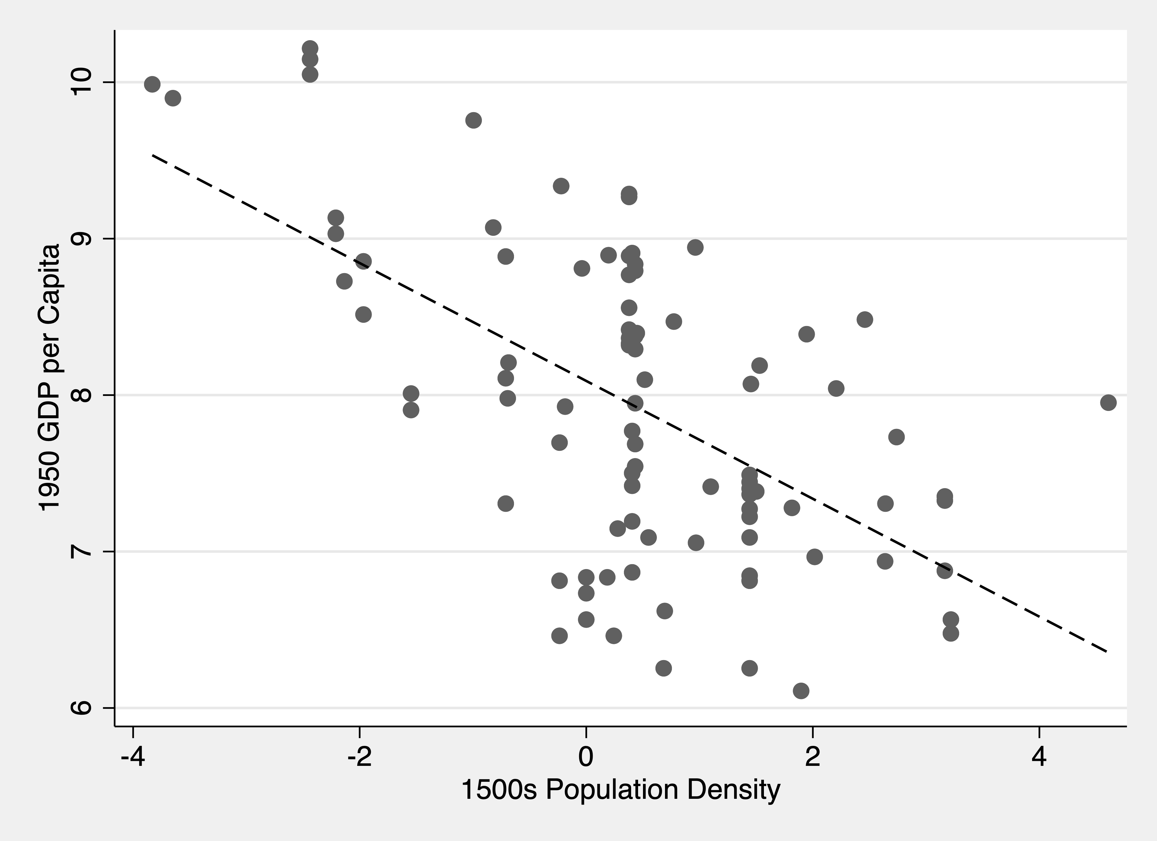
In this 2002 article, Acemoglu, Johnson, and Robinson argue that countries that were more wealthy and urbanized in the 1500s saw their fortunes reverse in the subsequent centuries. Countries such as Rwanda and Tanzania were high-density areas in the 1500s but in the 20th century had low GDP per capita. The authors argue that this is because European colonialism settled more in areas that were less developed in the 1500s, but then went on to become strong economies. A simple bivariate relationship motivates their argument.
. use reversal.dta, clear

. describe

Contains data from reversal.dta
  obs:            91
 vars:            10                          26 Nov 2018 22:42
 size:         7,553
───────────────────────────────────────────────────────────────────────────────────────────
              storage   display    value
variable name   type    format     label      variable label
───────────────────────────────────────────────────────────────────────────────────────────
countryn        str20   %-9s                  Country Name
shortnam        str3    %-9s                  Country Name
logpgp95        double  %10.0g                Log GDP per Capita in 1995
logem4          double  %10.0g
urbz1995        double  %10.0g                Urbanization in 1995 (Proportion Population
                                                in Large Towns)
lpd1500s        double  %10.0g                Log Population Density 1500s
cu1500          double  %10.0g                Urbanization in 1000s (Chandler)
sjb1500         double  %10.0g                Urbanization in 1500s (Bairoch)
sjb1000         double  %10.0g                Urbanization in 1000s (Bairoch)
continent       long    %8.0g      continent

───────────────────────────────────────────────────────────────────────────────────────────
Sorted by:
Use the regress or reg command to run a regression.
. regress logpgp95 lpd1500s

      Source │       SS           df       MS      Number of obs   =        91
─────────────┼──────────────────────────────────   F(1, 89)        =     46.12
       Model │  30.3661927         1  30.3661927   Prob > F        =    0.0000
    Residual │  58.5990948        89  .658416795   R-squared       =    0.3413
─────────────┼──────────────────────────────────   Adj R-squared   =    0.3339
       Total │  88.9652874        90  .988503194   Root MSE        =    .81143

─────────────┬────────────────────────────────────────────────────────────────
    logpgp95 │      Coef.   Std. Err.      t    P>|t|     [95% Conf. Interval]
─────────────┼────────────────────────────────────────────────────────────────
    lpd1500s │  -.3766786   .0554659    -6.79   0.000    -.4868881    -.266469
       _cons │   8.090425   .0887273    91.18   0.000     7.914126    8.266725
─────────────┴────────────────────────────────────────────────────────────────
In a simple regression, a scatter plot can show the data cleanly
. twoway scatter logpgp95 lpd1500s ||  lfit logpgp95 lpd1500s, ///
>    ytitle(1950 GDP per Capita) ///
>    xtitle(1500s Population Density) ///
>    legend(off)

. graph export reversal_fit.png, width(2000) replace
(file reversal_fit.png written in PNG format)
The Best Fit Regression Line
Different options:
. regress logpgp95 lpd1500s, beta

      Source │       SS           df       MS      Number of obs   =        91
─────────────┼──────────────────────────────────   F(1, 89)        =     46.12
       Model │  30.3661927         1  30.3661927   Prob > F        =    0.0000
    Residual │  58.5990948        89  .658416795   R-squared       =    0.3413
─────────────┼──────────────────────────────────   Adj R-squared   =    0.3339
       Total │  88.9652874        90  .988503194   Root MSE        =    .81143

─────────────┬────────────────────────────────────────────────────────────────
    logpgp95 │      Coef.   Std. Err.      t    P>|t|                     Beta
─────────────┼────────────────────────────────────────────────────────────────
    lpd1500s │  -.3766786   .0554659    -6.79   0.000                -.5842314
       _cons │   8.090425   .0887273    91.18   0.000                        .
─────────────┴────────────────────────────────────────────────────────────────
Multiple regression -- add more terms.
. reg logpgp95 lpd1500s sjb1000

      Source │       SS           df       MS      Number of obs   =        34
─────────────┼──────────────────────────────────   F(2, 31)        =     21.66
       Model │  14.2886648         2   7.1443324   Prob > F        =    0.0000
    Residual │  10.2267689        31  .329895772   R-squared       =    0.5828
─────────────┼──────────────────────────────────   Adj R-squared   =    0.5559
       Total │  24.5154337        33  .742891931   Root MSE        =    .57437

─────────────┬────────────────────────────────────────────────────────────────
    logpgp95 │      Coef.   Std. Err.      t    P>|t|     [95% Conf. Interval]
─────────────┼────────────────────────────────────────────────────────────────
    lpd1500s │   -.321548   .0551574    -5.83   0.000    -.4340423   -.2090538
     sjb1000 │  -.0031051   .0284966    -0.11   0.914    -.0612242     .055014
       _cons │   8.642748   .1485872    58.17   0.000     8.339703    8.945794
─────────────┴────────────────────────────────────────────────────────────────
What if explanatory variable is a categorical?
. tab continent

  continent │      Freq.     Percent        Cum.
────────────┼───────────────────────────────────
     Africa │         45       49.45       49.45
   Americas │         32       35.16       84.62
       Asia │         12       13.19       97.80
    Oceania │          2        2.20      100.00
────────────┼───────────────────────────────────
      Total │         91      100.00
. reg logpgp95 lpd1500s sjb1000 continent

      Source │       SS           df       MS      Number of obs   =        34
─────────────┼──────────────────────────────────   F(3, 30)        =     13.97
       Model │  14.2889201         3  4.76297337   Prob > F        =    0.0000
    Residual │  10.2265136        30  .340883787   R-squared       =    0.5829
─────────────┼──────────────────────────────────   Adj R-squared   =    0.5411
       Total │  24.5154337        33  .742891931   Root MSE        =    .58385

─────────────┬────────────────────────────────────────────────────────────────
    logpgp95 │      Coef.   Std. Err.      t    P>|t|     [95% Conf. Interval]
─────────────┼────────────────────────────────────────────────────────────────
    lpd1500s │  -.3212955   .0568227    -5.65   0.000     -.437343    -.205248
     sjb1000 │  -.0028831   .0300819    -0.10   0.924    -.0643186    .0585524
   continent │   .0041495   .1516197     0.03   0.978    -.3054991    .3137982
       _cons │   8.632706   .3968173    21.75   0.000     7.822297    9.443115
─────────────┴────────────────────────────────────────────────────────────────
(what's wrong with this?)
. reg logpgp95 lpd1500s sjb1000 i.continent

      Source │       SS           df       MS      Number of obs   =        34
─────────────┼──────────────────────────────────   F(5, 28)        =     11.84
       Model │  16.6431982         5  3.32863964   Prob > F        =    0.0000
    Residual │  7.87223551        28  .281151268   R-squared       =    0.6789
─────────────┼──────────────────────────────────   Adj R-squared   =    0.6215
       Total │  24.5154337        33  .742891931   Root MSE        =    .53024

─────────────┬────────────────────────────────────────────────────────────────
    logpgp95 │      Coef.   Std. Err.      t    P>|t|     [95% Conf. Interval]
─────────────┼────────────────────────────────────────────────────────────────
    lpd1500s │  -.4108716   .0664944    -6.18   0.000    -.5470792   -.2746641
     sjb1000 │    .017904   .0287151     0.62   0.538    -.0409162    .0767241
             │
   continent │
   Americas  │  -.9076474   .3537367    -2.57   0.016    -1.632244   -.1830505
       Asia  │  -.5490911   .3531067    -1.56   0.131    -1.272397    .1742151
    Oceania  │  -.3875177    .548546    -0.71   0.486    -1.511163    .7361279
             │
       _cons │   9.260819   .3231567    28.66   0.000     8.598863    9.922776
─────────────┴────────────────────────────────────────────────────────────────
Create a new variable in dataset
. reg logpgp95 lpd1500s sjb1000 i.continent

      Source │       SS           df       MS      Number of obs   =        34
─────────────┼──────────────────────────────────   F(5, 28)        =     11.84
       Model │  16.6431982         5  3.32863964   Prob > F        =    0.0000
    Residual │  7.87223551        28  .281151268   R-squared       =    0.6789
─────────────┼──────────────────────────────────   Adj R-squared   =    0.6215
       Total │  24.5154337        33  .742891931   Root MSE        =    .53024

─────────────┬────────────────────────────────────────────────────────────────
    logpgp95 │      Coef.   Std. Err.      t    P>|t|     [95% Conf. Interval]
─────────────┼────────────────────────────────────────────────────────────────
    lpd1500s │  -.4108716   .0664944    -6.18   0.000    -.5470792   -.2746641
     sjb1000 │    .017904   .0287151     0.62   0.538    -.0409162    .0767241
             │
   continent │
   Americas  │  -.9076474   .3537367    -2.57   0.016    -1.632244   -.1830505
       Asia  │  -.5490911   .3531067    -1.56   0.131    -1.272397    .1742151
    Oceania  │  -.3875177    .548546    -0.71   0.486    -1.511163    .7361279
             │
       _cons │   9.260819   .3231567    28.66   0.000     8.598863    9.922776
─────────────┴────────────────────────────────────────────────────────────────

. predict yhat
(option xb assumed; fitted values)
(57 missing values generated)

. summarize logpgp95 yhat

    Variable │        Obs        Mean    Std. Dev.       Min        Max
─────────────┼─────────────────────────────────────────────────────────
    logpgp95 │         91    7.918999     .994235   6.109248   10.21574
        yhat │         34    8.614128    .7101685   7.443351   10.37231
Or residuals
. predict residuals, residuals
(57 missing values generated)

.
. summarize logpgp95 yhat residuals

    Variable │        Obs        Mean    Std. Dev.       Min        Max
─────────────┼─────────────────────────────────────────────────────────
    logpgp95 │         91    7.918999     .994235   6.109248   10.21574
        yhat │         34    8.614128    .7101685   7.443351   10.37231
   residuals │         34   -2.74e-09    .4884185  -1.083866   .8918947
Instead of copy-pasting Stata output, use designated commands:
. reg logpgp95 lpd1500s sjb1000

      Source │       SS           df       MS      Number of obs   =        34
─────────────┼──────────────────────────────────   F(2, 31)        =     21.66
       Model │  14.2886648         2   7.1443324   Prob > F        =    0.0000
    Residual │  10.2267689        31  .329895772   R-squared       =    0.5828
─────────────┼──────────────────────────────────   Adj R-squared   =    0.5559
       Total │  24.5154337        33  .742891931   Root MSE        =    .57437

─────────────┬────────────────────────────────────────────────────────────────
    logpgp95 │      Coef.   Std. Err.      t    P>|t|     [95% Conf. Interval]
─────────────┼────────────────────────────────────────────────────────────────
    lpd1500s │   -.321548   .0551574    -5.83   0.000    -.4340423   -.2090538
     sjb1000 │  -.0031051   .0284966    -0.11   0.914    -.0612242     .055014
       _cons │   8.642748   .1485872    58.17   0.000     8.339703    8.945794
─────────────┴────────────────────────────────────────────────────────────────

. esttab

────────────────────────────
                      (1)
                 logpgp95
────────────────────────────
lpd1500s           -0.322***
                  (-5.83)

sjb1000          -0.00311
                  (-0.11)

_cons               8.643***
                  (58.17)
────────────────────────────
N                      34
────────────────────────────
t statistics in parentheses
* p<0.05, ** p<0.01, *** p<0.001

.
. eststo clear // clear estimated tables

. eststo: reg logpgp95 lpd1500s

      Source │       SS           df       MS      Number of obs   =        91
─────────────┼──────────────────────────────────   F(1, 89)        =     46.12
       Model │  30.3661927         1  30.3661927   Prob > F        =    0.0000
    Residual │  58.5990948        89  .658416795   R-squared       =    0.3413
─────────────┼──────────────────────────────────   Adj R-squared   =    0.3339
       Total │  88.9652874        90  .988503194   Root MSE        =    .81143

─────────────┬────────────────────────────────────────────────────────────────
    logpgp95 │      Coef.   Std. Err.      t    P>|t|     [95% Conf. Interval]
─────────────┼────────────────────────────────────────────────────────────────
    lpd1500s │  -.3766786   .0554659    -6.79   0.000    -.4868881    -.266469
       _cons │   8.090425   .0887273    91.18   0.000     7.914126    8.266725
─────────────┴────────────────────────────────────────────────────────────────
(est1 stored)

. eststo: reg logpgp95 lpd1500s sjb1000

      Source │       SS           df       MS      Number of obs   =        34
─────────────┼──────────────────────────────────   F(2, 31)        =     21.66
       Model │  14.2886648         2   7.1443324   Prob > F        =    0.0000
    Residual │  10.2267689        31  .329895772   R-squared       =    0.5828
─────────────┼──────────────────────────────────   Adj R-squared   =    0.5559
       Total │  24.5154337        33  .742891931   Root MSE        =    .57437

─────────────┬────────────────────────────────────────────────────────────────
    logpgp95 │      Coef.   Std. Err.      t    P>|t|     [95% Conf. Interval]
─────────────┼────────────────────────────────────────────────────────────────
    lpd1500s │   -.321548   .0551574    -5.83   0.000    -.4340423   -.2090538
     sjb1000 │  -.0031051   .0284966    -0.11   0.914    -.0612242     .055014
       _cons │   8.642748   .1485872    58.17   0.000     8.339703    8.945794
─────────────┴────────────────────────────────────────────────────────────────
(est2 stored)

. eststo: reg logpgp95 lpd1500s sjb1000 i.continent

      Source │       SS           df       MS      Number of obs   =        34
─────────────┼──────────────────────────────────   F(5, 28)        =     11.84
       Model │  16.6431982         5  3.32863964   Prob > F        =    0.0000
    Residual │  7.87223551        28  .281151268   R-squared       =    0.6789
─────────────┼──────────────────────────────────   Adj R-squared   =    0.6215
       Total │  24.5154337        33  .742891931   Root MSE        =    .53024

─────────────┬────────────────────────────────────────────────────────────────
    logpgp95 │      Coef.   Std. Err.      t    P>|t|     [95% Conf. Interval]
─────────────┼────────────────────────────────────────────────────────────────
    lpd1500s │  -.4108716   .0664944    -6.18   0.000    -.5470792   -.2746641
     sjb1000 │    .017904   .0287151     0.62   0.538    -.0409162    .0767241
             │
   continent │
   Americas  │  -.9076474   .3537367    -2.57   0.016    -1.632244   -.1830505
       Asia  │  -.5490911   .3531067    -1.56   0.131    -1.272397    .1742151
    Oceania  │  -.3875177    .548546    -0.71   0.486    -1.511163    .7361279
             │
       _cons │   9.260819   .3231567    28.66   0.000     8.598863    9.922776
─────────────┴────────────────────────────────────────────────────────────────
(est3 stored)

. esttab

────────────────────────────────────────────────────────────
                      (1)             (2)             (3)
                 logpgp95        logpgp95        logpgp95
────────────────────────────────────────────────────────────
lpd1500s           -0.377***       -0.322***       -0.411***
                  (-6.79)         (-5.83)         (-6.18)

sjb1000                          -0.00311          0.0179
                                  (-0.11)          (0.62)

1.continent                                             0
                                                      (.)

2.continent                                        -0.908*
                                                  (-2.57)

3.continent                                        -0.549
                                                  (-1.56)

4.continent                                        -0.388
                                                  (-0.71)

_cons               8.090***        8.643***        9.261***
                  (91.18)         (58.17)         (28.66)
────────────────────────────────────────────────────────────
N                      91              34              34
────────────────────────────────────────────────────────────
t statistics in parentheses
* p<0.05, ** p<0.01, *** p<0.001
With more formats (http://repec.org/bocode/e/estout/esttab.html)
. esttab, label b(2) se(a1) r2 ar2

────────────────────────────────────────────────────────────────────
                              (1)             (2)             (3)
                     Log GDP~1995    Log GDP~1995    Log GDP~1995
────────────────────────────────────────────────────────────────────
Log Population~1500s        -0.38***        -0.32***        -0.41***
                           (0.06)          (0.06)          (0.07)

Urbanization in 10~)                        -0.00            0.02
                                           (0.03)          (0.03)

Africa                                                       0.00
                                                              (.)

Americas                                                    -0.91*
                                                            (0.4)

Asia                                                        -0.55
                                                            (0.4)

Oceania                                                     -0.39
                                                            (0.5)

Constant                     8.09***         8.64***         9.26***
                           (0.09)           (0.1)           (0.3)
────────────────────────────────────────────────────────────────────
Observations                   91              34              34
R-squared                   0.341           0.583           0.679
Adjusted R-squared          0.334           0.556           0.622
────────────────────────────────────────────────────────────────────
Standard errors in parentheses
* p<0.05, ** p<0.01, *** p<0.001