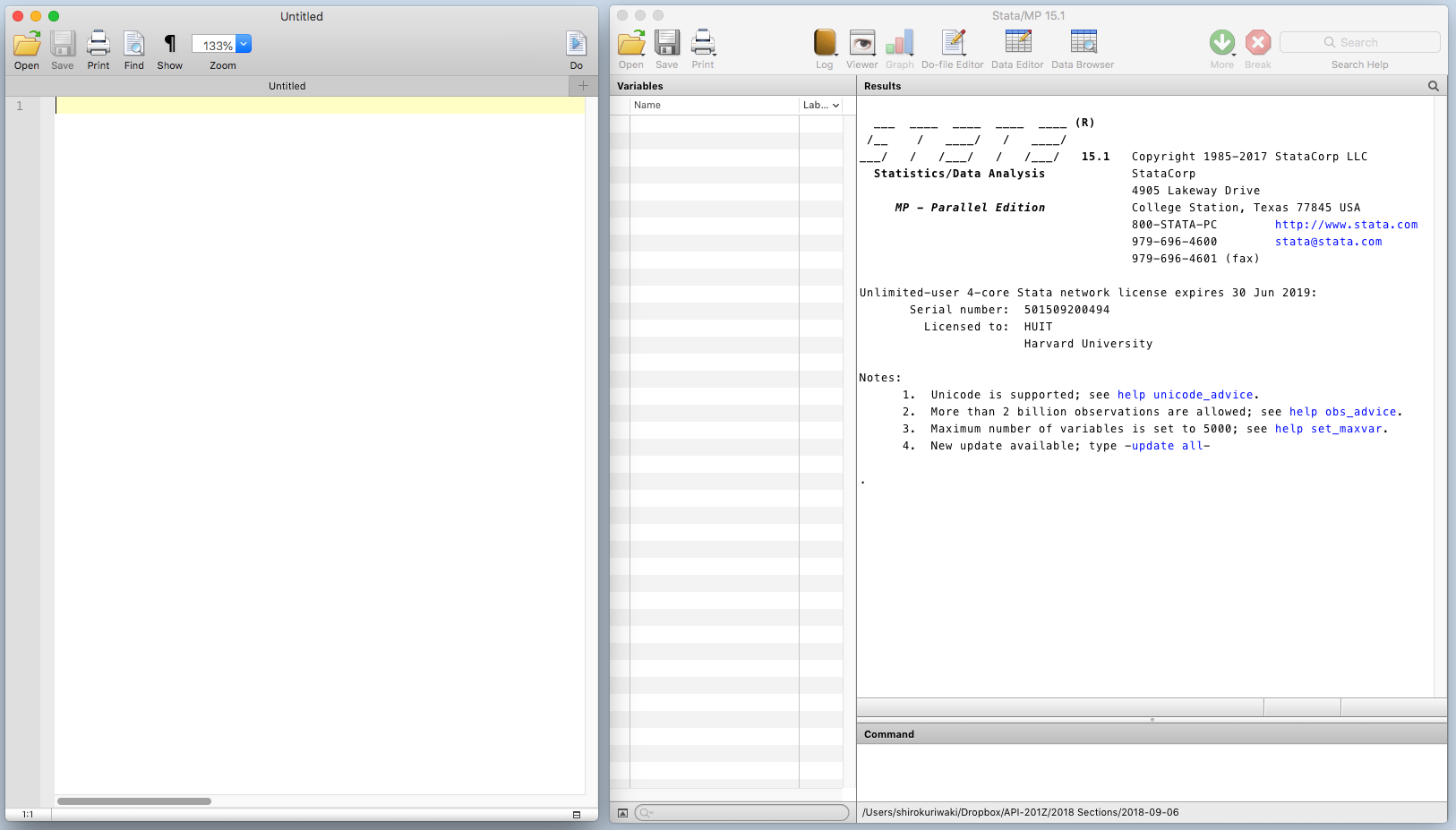
What's what in a Stata Window
How does one "do Stata"? We interact with Stata by sending the statistical program "commands". Commands can be anything from reading in a dataset to running a regression.
What's what in a Stata Window
Stata takes one dataset at a time and runs manipulations on it. To clear the memory (i.e. the dataset and other auxilarly objects) in Stata, the command is:
clear allFor the above code and all other Stata code in this document, you can run it after removing the period . in the beginning -- which indicates a command that was already entered.
If you know the name of the function you want to use but aren't sure how to use it, use the help command by typing in help and then the name of the function.
help ivregressIf you do not know the exact name of the function, you can Google or search on Stata's help manual / search box.
Stata commands are stored in a script. You can write commands directly into the command window to get similar results. However, it is often a bad idea to do your analysis through the command window because it is easy to forget the exact steps. Instead, you should save your commands in a script -- a .do file. When we ask for scripts on problem sets, we are looking for a script.
The .do file lacks a way to store the output of your commands. To store output you can generate a separate log file along with your .do scripts. To do so,
start your .do file with
log using kuriwaki_log.txt, text replacewhere the filename kuriwaki_log.txt can be replaced by any name of your choice.
Then at the end of your .do file, enter
log closeto close the log.
Finally, you also might want to enter at the very first line, before log using..., the following
capture log closeto close any already opened logs (if they exist).
When working in Stata, it's always an important first step to make sure you're in the right working directory (where you tell Stata what folder you want to work in).
pwd stands for "present working directory". cd stands for "change directory". ls stands for "list (the files in current directory)". . is shorthand for the current directory, .. for the parent directory, and ~/ for your home directory.
For example,
cd "~/Dropbox/temp"You will want to modify the path above to your own.
Now, load the .dta file provided into Stata:
. use sample_data.dta
Note that use is limited to .dta files; Stata's designated way of storing datasets. The most useful feature of a .dta format is that the data values comes with labels. For example, a .dta will be able to store the fact that the labels female and male correspond to values 1 and 2, respectively.
Sometimes, your data will not come in a .dta format. A basic format is .csv -- standing for comma-separated-values. These files is like an Excel spreadsheet, but without any of the formatting (color, functions, comments). The csv is a common and desirable form in programming, as it can be read by any statistical program.
What if we needed to load a csv file?
. import delimited using sample_data.csv, clear
(7 vars, 435 obs)
We see that compared to the one-word use, the Stata syntax is a bit more lengthy to read in a spreadsheet. Again, enter help import or help import delimited to understand thi son your own. The help page tells us that we use import delimited and then the file name followed by the using word.
You will see the comma used many times in Stata code. On the left-side of the comma, you put the main command. On the right-side, you put secondary options. The comma often confuses first-time users.
. clear all
To go through how to analyze and review data, let's work with a dataset that is pre-loaded into the Stata app.
The command sysuse is a command to use a data already baked into the system. Then nlsw88 is one of the several datasets that are available.
This is an extract from the 1988 National Longitudinal Survey of Women, which is a survey conducted by the Department of Labor. This extract contains about 2000 women in their 30s and 40s.
. sysuse nlsw88
(NLSW, 1988 extract)
To look at the data we've just loaded in, use the command browse (or br for short):
browseTo get a list of the variables and the variable types:
. describe

Contains data from /Applications/Stata/ado/base/n/nlsw88.dta
  obs:         2,246                          NLSW, 1988 extract
 vars:            17                          1 May 2016 22:52
 size:        60,642                          (_dta has notes)
──────────────────────────────────────────────────────────────────────────────────
              storage   display    value
variable name   type    format     label      variable label
──────────────────────────────────────────────────────────────────────────────────
idcode          int     %8.0g                 NLS id
age             byte    %8.0g                 age in current year
race            byte    %8.0g      racelbl    race
married         byte    %8.0g      marlbl     married
never_married   byte    %8.0g                 never married
grade           byte    %8.0g                 current grade completed
collgrad        byte    %16.0g     gradlbl    college graduate
south           byte    %8.0g                 lives in south
smsa            byte    %9.0g      smsalbl    lives in SMSA
c_city          byte    %8.0g                 lives in central city
industry        byte    %23.0g     indlbl     industry
occupation      byte    %22.0g     occlbl     occupation
union           byte    %8.0g      unionlbl   union worker
wage            float   %9.0g                 hourly wage
hours           byte    %8.0g                 usual hours worked
ttl_exp         float   %9.0g                 total work experience
tenure          float   %9.0g                 job tenure (years)
──────────────────────────────────────────────────────────────────────────────────
Sorted by: idcode
We can see that there are seventeen variables in this dataset.
. sum age

    Variable │        Obs        Mean    Std. Dev.       Min        Max
─────────────┼─────────────────────────────────────────────────────────
         age │      2,246    39.15316    3.060002         34         46
. sum age, detail

                     age in current year
─────────────────────────────────────────────────────────────
      Percentiles      Smallest
 1%           34             34
 5%           35             34
10%           35             34       Obs               2,246
25%           36             34       Sum of Wgt.       2,246

50%           39                      Mean           39.15316
                        Largest       Std. Dev.      3.060002
75%           42             45
90%           44             45       Variance       9.363614
95%           44             46       Skewness       .2003234
99%           45             46       Kurtosis       1.932389
. tabstat age, stat(mean sd median iqr)

    variable │      mean        sd       p50       iqr
─────────────┼────────────────────────────────────────
         age │  39.15316  3.060002        39         6
─────────────┴────────────────────────────────────────
To create a new variable, use the generate (gen for short) command:
. gen weekly_wage = wage * hours
(4 missing values generated)
Stata, along with SPSS, adds "labels" to variables. You might think of the labels as "pretty names" that are more legible than "weekly_wage". labels show up in the Stata variable window and are also get used in graphs. It is often worth the extra effort to label your own variables.
. label variable weekly_wage "weekly wage (estimate)"
If you want to redefine a variable, use the replace command:
. gen foo = (age)^2

. replace foo = 0
(2,246 real changes made)
To "drop" (delete) a variable:
. drop foo
To count the rows in your dataset,
. count
  2,246
What about counting only observations that match a certain condition? Use if at the end and the boolean conditions ==, !=, |, and &.
. count if south == 1
  942
tabulate is an oft-used function for counting. We can either do a one-way or two-way tabulation.
One-way tabs is a tabulation of counts
. tabulate c_city

   lives in │
    central │
       city │      Freq.     Percent        Cum.
────────────┼───────────────────────────────────
          0 │      1,591       70.84       70.84
          1 │        655       29.16      100.00
────────────┼───────────────────────────────────
      Total │      2,246      100.00
Two-way tabs is referred to as a "crosstab"
. tabulate c_city union

  lives in │
   central │     union worker
      city │  nonunion      union │     Total
───────────┼──────────────────────┼──────────
         0 │     1,034        288 │     1,322
         1 │       383        173 │       556
───────────┼──────────────────────┼──────────
     Total │     1,417        461 │     1,878
First, I strongly recommend you re-set your default color palette
. set scheme s2mono, permanently
(set scheme preference recorded)
which just makes for simpler and better looking plots.
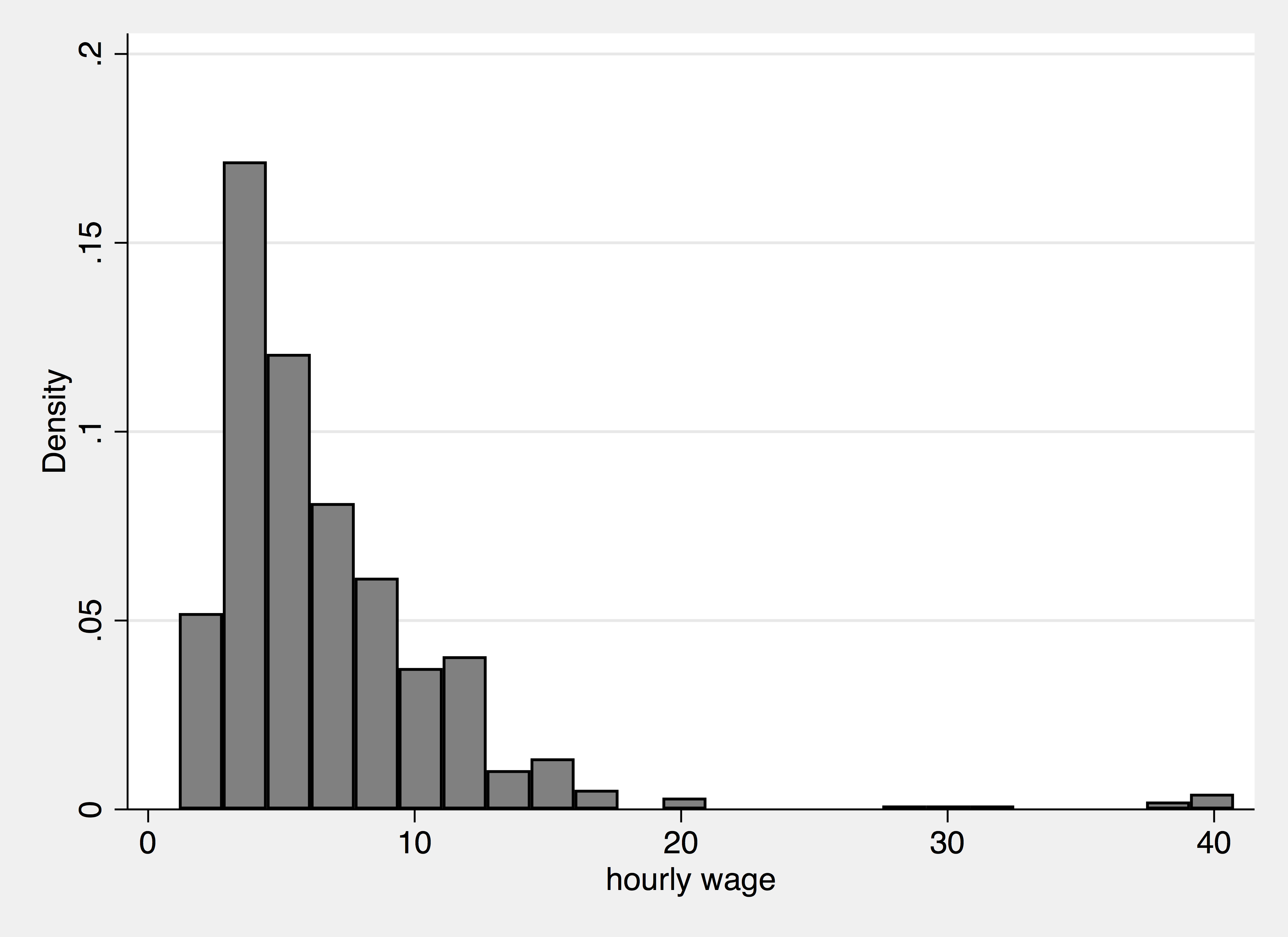
The hist command will generate a histogram.
. hist wage
(bin=33, start=1.0049518, width=1.2042921)

. graph export hist_wage.png, width(2000) replace
(file hist_wage.png written in PNG format)
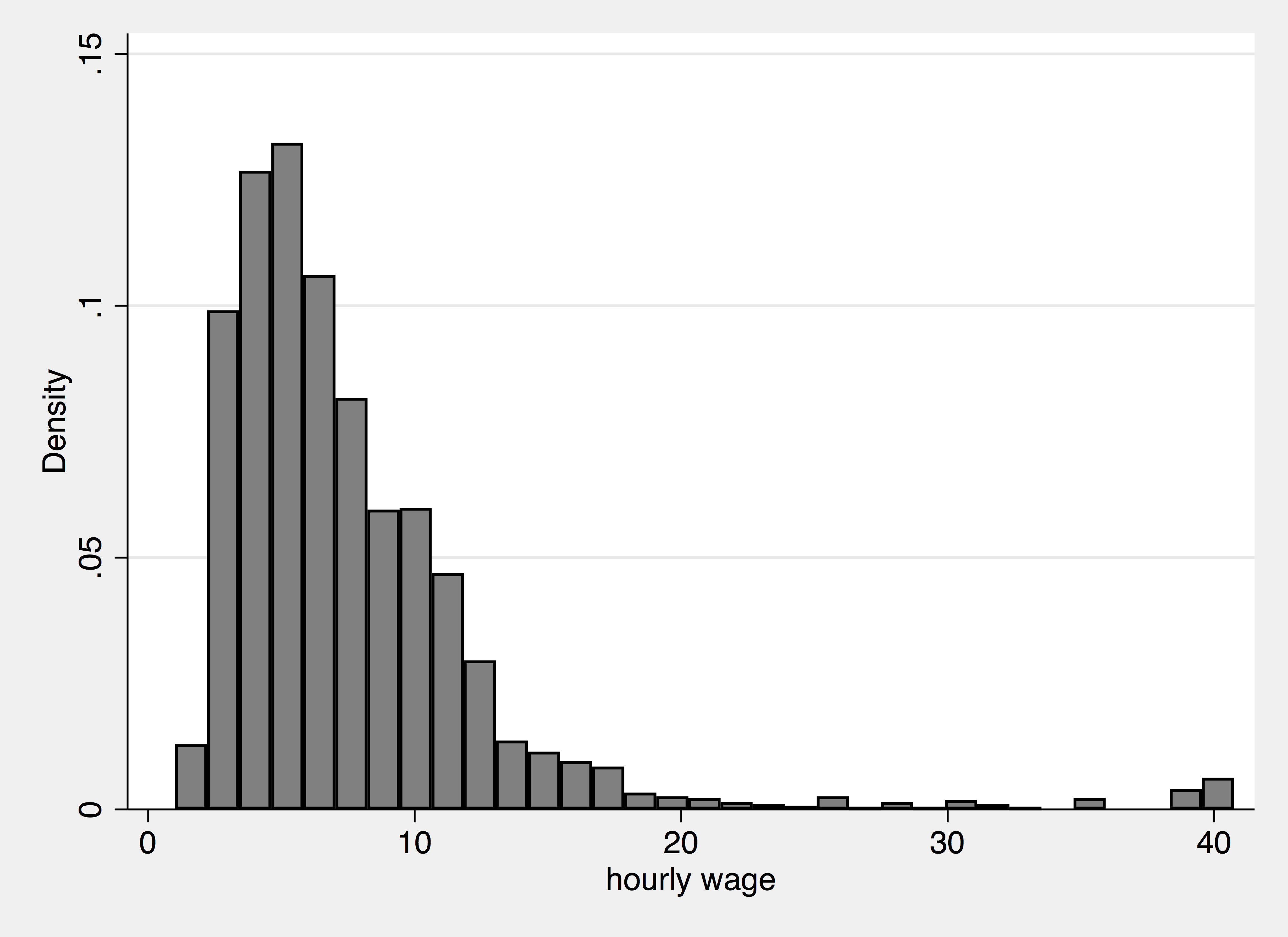
A Histogram
Note that we have two commands -- hist and graph export. The first generates the figure within Stata; the second saves that figure as a file on your computer. Saving files will be make your workflow easier than saving files through the click-and-drag interface each time.
The scatter command will generate a scatterplot. Two variables...two dimensions. The y-variable comes first, then the x-variable:
. scatter weekly_wage grade

. graph export edu_wage.png, width(1800) replace
(file edu_wage.png written in PNG format)
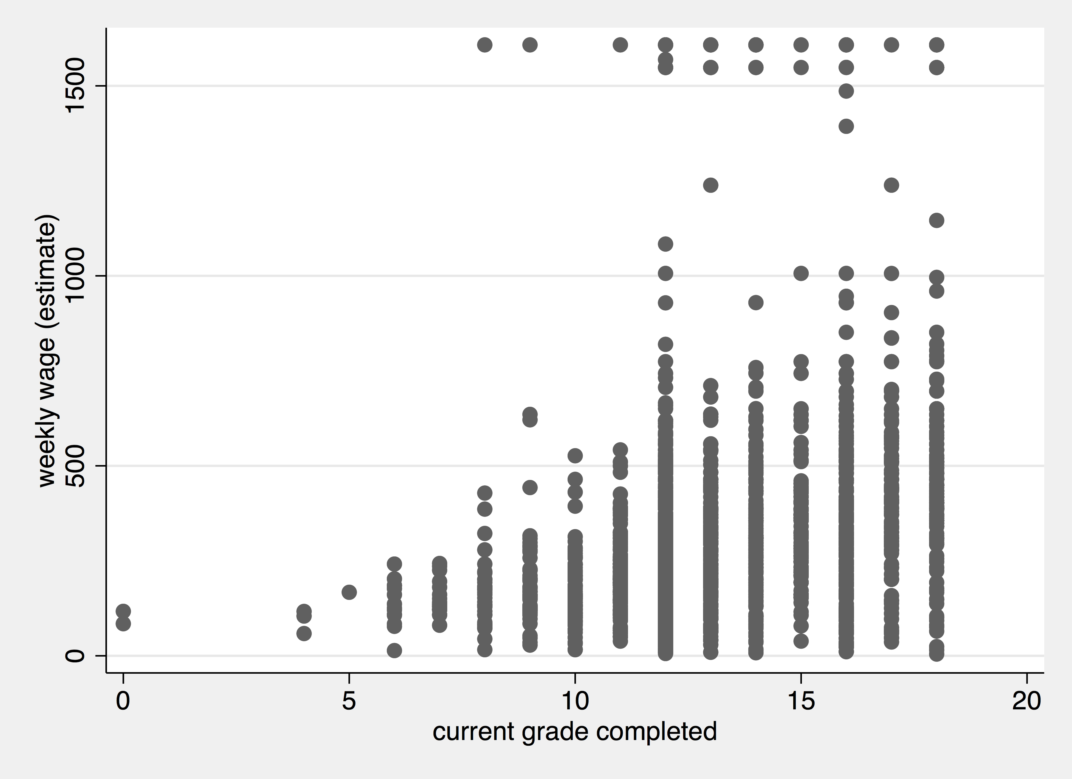
A Scatter Plot
The graph export has many options beyond the default, and they come after a comma ,. Again, this is a general Stata rule -- options come after a comma. Like all commands, use the command help (as in help graph export) to see all of them.
For example, we notice that the points above are overlapping and it is hard to distinguish whether a point overlap with one other point or 100s of other points. To this we could make the points transparent.
. scatter weekly_wage grade, mcolor(%30)

. graph export edu_wage_alpha.png, width(1800) replace
(file edu_wage_alpha.png written in PNG format)
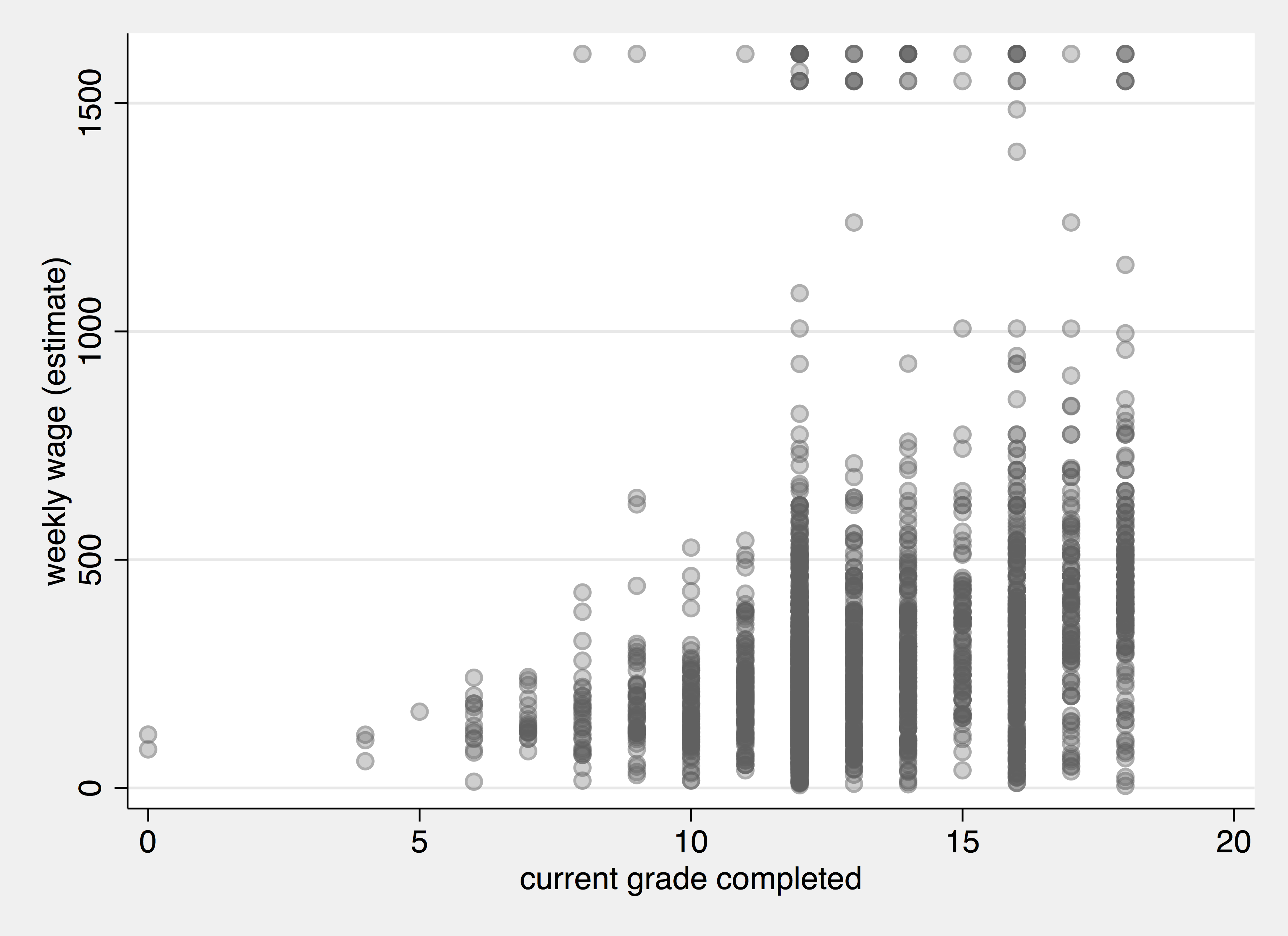
A Scatter Plot + Transparency
What if we only wanted to plot the wage of of blacks? We want to use a conditional "if" statement:
. hist wage if race == "black":racelbl
(bin=24, start=1.1513683, width=1.6498009)

. graph export wage_blk.png, width(2000) replace
(file wage_blk.png written in PNG format)
Scatter Plot + If
To compare the distribution of the same variable across groups, a boxplot is useful
. graph box wage, over(race)

. graph export race_wage.png, width(2000) replace
(file race_wage.png written in PNG format)
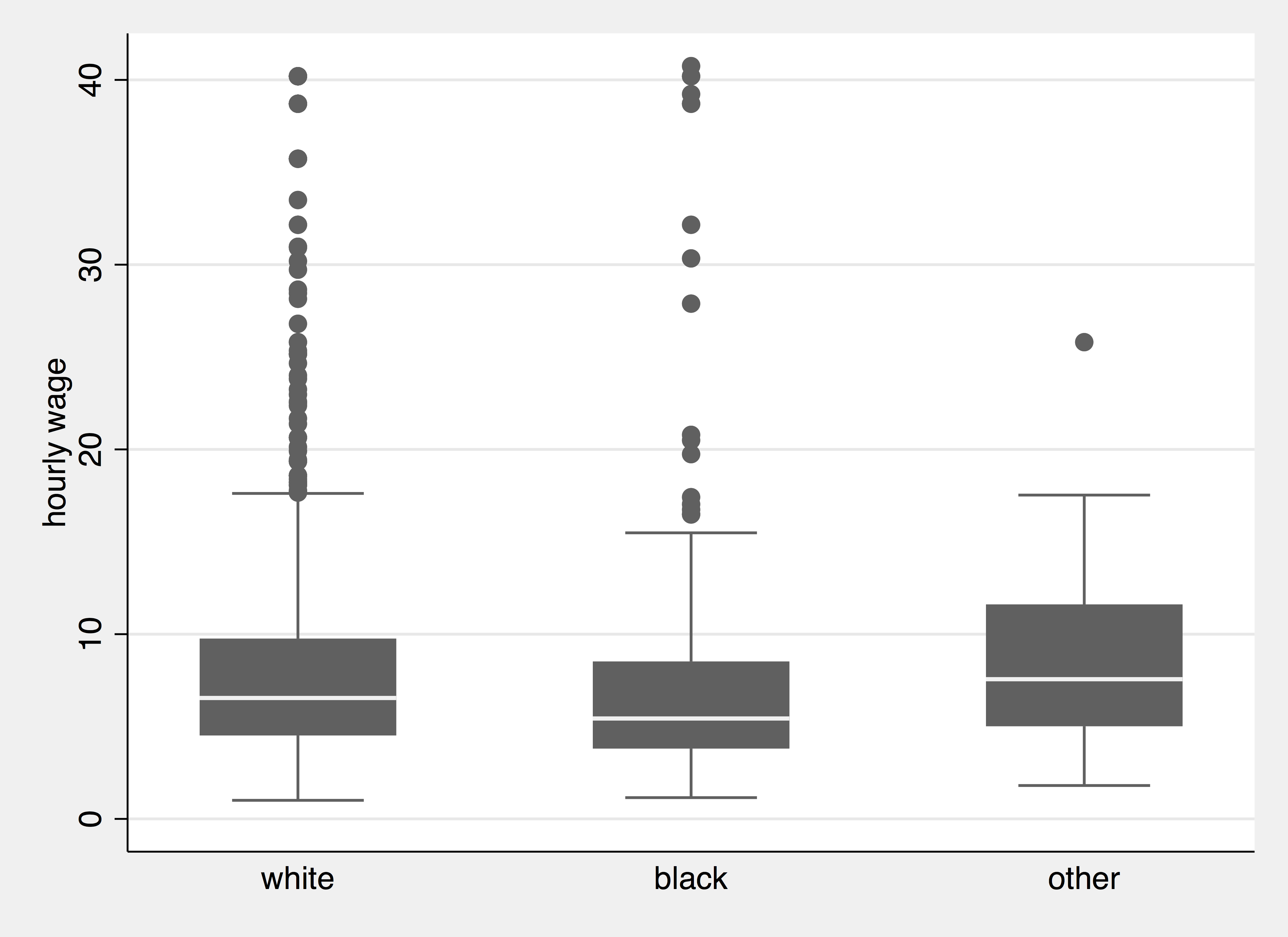
Boxplot
What if we wanted to plot these two last scatterplots side-by-side? We can give each one a name and then combine them:
. scatter weekly_wage grade if race == "black":racelbl, ///
>    title("Black Women") name(blk_edu_wage, replace)

. scatter weekly_wage grade if race == "white":racelbl, ///
>    title("White Women") name(wht_edu_wage, replace)

. graph combine blk_edu_wage wht_edu_wage, ysize(2) xsize(3)

. graph export race_edu_wage.png, width(2000) replace
(file race_edu_wage.png written in PNG format)
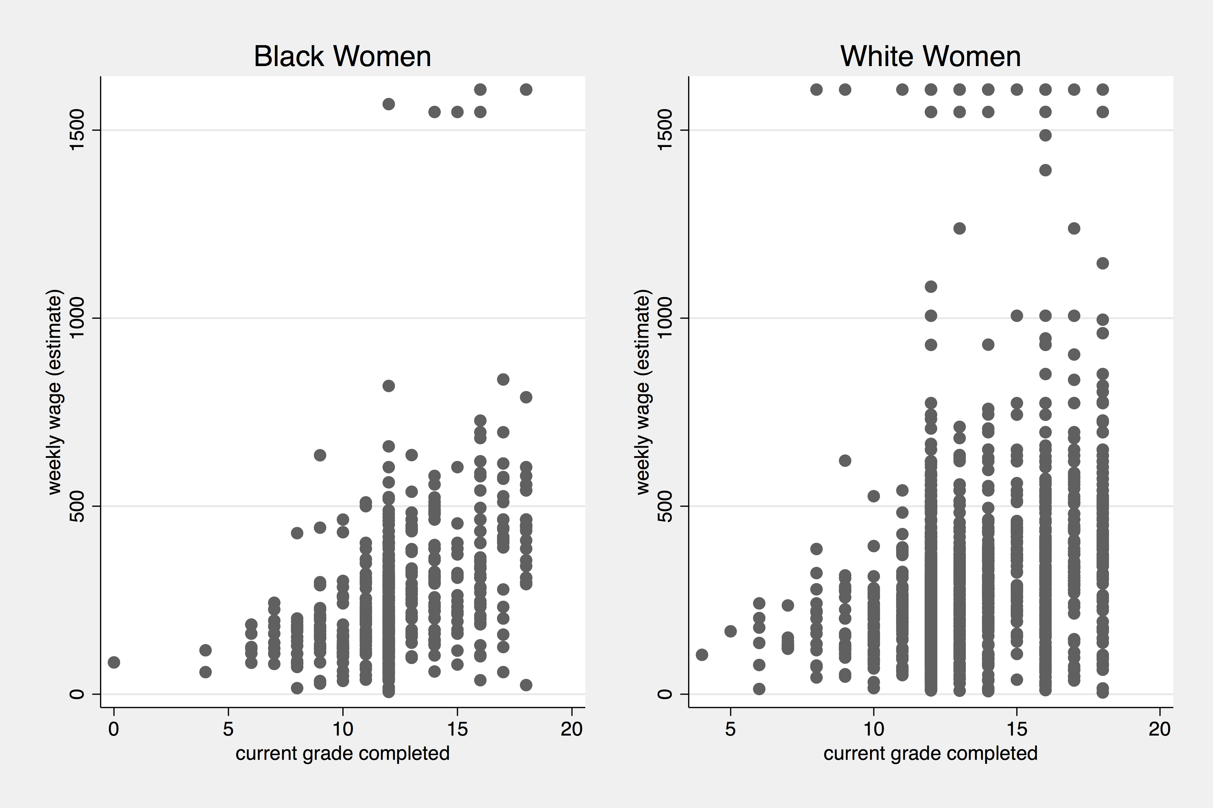
Scatter Plot side-by-side
Unless you are already a Stata flow you will probably need to constantly refer to online and Stata-based resources on the command names and syntax of the commands you'd want to run. The Stata manual enclosed in the Stata Application and online message boards are helpful. A nice cheat-sheet of commands is here https://geocenter.github.io/StataTraining/pdf/AllCheatSheets.pdf
and is also uploaded on Canvas (https://canvas.harvard.edu/courses/52520/files/folder/Programming-Resources)
help set scheme) or others such as those by Daniel Bischoff: https://www.stata.com/meeting/switzerland16/slides/bischof-switzerland16.pdfFor compilation, I used the markstat package by Germán Rodríguez. http://data.princeton.edu/stata/markdown. Source Code: https://github.com/kuriwaki/stata-notes. Contact: Shiro Kuriwaki, kuriwaki@g.harvard.edu